

Sparsity in Weight Space: What Does LLM Post-Training Change?
Primary sources
This article is a close reading of the following three papers. Each was read in full, including its appendices.
| Paper | Authors | Date | In this article | |
|---|---|---|---|---|
| A | Understanding LLM Parameter Update Sparsity through the Lens of Fisher | Yufan Zhang, Sagnik Mukherjee, Hao Peng | 28 September 2026 | Section 4 |
| B | Not How Many, But Which: Parameter Placement in Low-Rank Adaptation | Arijit Sehanobish, Charles Lovering | 12 May 2026 | Section 5 |
| C | The Surprising Effectiveness of Deleting Weights in LLM Post-Training | Jack Lu, Zhenbang Yang, Mike Lasby, Tejas Pote, Yani Ioannou, Mengye Ren | 7 November 2026, NeurIPS 2026 | Section 6 |
Supplementary source: Sparks of Weight-Space Programming (Takehi, Teoh, Zhang, Khattab; MIT CSAIL blog post, 2 November 2026), Section 7. Since it is not a peer-reviewed paper, it is not given the same evidential weight as the three primary sources.
Three kinds of material are kept distinct throughout: what the papers say, with citations; our interpretation, marked as “our reading” or a “hypothesis”; and a small-scale verification experiment conducted for this article (Section 8).
A note on terminology: the Turkish original retains established technical terms in English, including weight space, attention, head, gate, residual stream, fine-tuning, pruning, baseline, forward pass, learning rate, seed, and on-policy. Words with established everyday equivalents, such as weight, layer, gradient, mask, reward, training, and forgetting, are expressed in Turkish there.
How to read this article
The article is intended for both newcomers and readers familiar with the topic. There are three routes:
15 minutes. Read the summary, Section 9, and the balance sheet in Section 8.9. These cover the main thesis, the contradictions, and the new finding.
Practitioner. Read Section 2.0, then Sections 5, 8, and 11. These explain which parameters to select and which experiment to run first.
Full reading. Read from beginning to end. If softmax, gradients, or Adam are unfamiliar, do not skip Section 2.0; consult the glossary at the end when you encounter an unfamiliar term.
Summary
When a language model is trained with reinforcement learning (RL), or on data close to its own distribution, only a very small fraction of its billions of weights changes meaningfully. Three papers published in 2026 examine this observation from three directions. Read together, they suggest the following picture: post-training does not load large amounts of knowledge into a model; it adjusts how the model uses capabilities it already has, and that adjustment lives in a small, predictable set of weights.
This article closely reads those three papers, with a fourth source treated as supplementary:
Why sparse? Zhang, Mukherjee, and Peng show that diagonal Fisher information bounds the expected gradient. A weight that does not affect the output distribution receives no gradient either.
Which weights? By training only a few thousand entries in LoRA’s B matrix, Sehanobish and Lovering show that placement is decisive under RL, whereas under SFT it matters very little.
How little? Without changing the values of the remaining weights, Lu and colleagues match full fine-tuning accuracy in models of 7B and above by deleting fewer than 0.05% of weights.
Are gradients necessary? Takehi and colleagues offer early evidence that a strong LLM can read weights and edit them directly.
The article adds four things to the papers. First, a contradiction none of the three discusses: random sparse selection learns nothing in A and B, yet matches full fine-tuning in C (Section 9.3). Second, a verification experiment in a 75,000-parameter model: four claims held and four did not, and a Fisher-selected mask performed worse than a random mask when teaching the model something new (Section 8). Third, a short derivation connecting A’s Fisher bound to B’s gradient score through Adam (Section 9.4). Fourth, six experiments to test the questions left open (Section 11).
Reading note: all numbers in Sections 4–7 come from the sources; those in Section 8 come from the experiment conducted for this article. Interpretations and inferences are explicitly marked as “our reading” or a “hypothesis.”
1. Introduction
When we think of fine-tuning a model, the usual picture is this: the optimizer nudges every weight, moving the model somewhere new. Full fine-tuning (FFT) takes this picture literally and produces a new 30 GB checkpoint for an 8B model. LoRA narrows it somewhat: the update lives in a low-rank subspace. Both assume that the update is spread across the weights.
In 2025, an observation challenged this assumption. Mukherjee and colleagues compared publicly available RL checkpoints on Hugging Face with their base models and found that 68.5% to 96% of weights had not changed at all. This recurred across seven RL algorithms and ten models, spontaneously, without sparsity regularization. More interestingly, the subnetworks that changed overlapped across seeds, datasets, and even algorithms far more than chance would explain. And although the update was sparse, it was not low-rank: few weights changed, but they spanned almost the matrix’s entire subspace.
This observation raises three questions at once:
Mechanism. The optimizer computes a gradient for every weight. Why do most receive a near-zero gradient?
Location. Can we predict which weights will change before training? If so, is training only those weights sufficient?
Lower bound. How small can the required change become? Must a weight acquire a new value, or is silencing it enough?
Three papers published between May and November 2026 address these questions in turn. A fourth, a blog post, changes the question itself: if the weights determining behavior form such a small, identifiable set, do we need gradients to find it?
Why it matters
Beyond academic curiosity, the topic has four practical implications.
Deployment cost. If a task-specific change fits in a mask of a few megabytes, hundreds of specialized variants can share one base model.
Forgetting. If most weights remain untouched, much of the model’s previous knowledge is preserved. This is a property continual learning has sought for years.
Interpretability. If a behavioral change lives in 10,000 weights, examining those weights is far more realistic than examining 8 billion.
Small models and limited hardware. If the trainable parameter count falls by five orders of magnitude, RL post-training becomes feasible on a single consumer GPU.
Road map
Section 2 establishes the necessary concepts: weight space, post-training regimes, and transformer-block projections. Section 3 traces the roots of today’s results in pruning research. Sections 4–7 examine the four sources individually, at the level of methods and evidence. Section 8 tests the papers’ main claims from scratch in a small model. Section 9 brings them together and discusses their disagreements. Section 10 sets out the open questions, and Section 11 proposes experiments to test them.
2. Background
This section establishes the concepts used throughout: first five basic ideas (2.0), then five topic-specific areas (2.1–2.5). Readers familiar with the subject can go straight to Section 3.
2.0 Prerequisites: five basic concepts
This subsection is for newcomers. The rest of the article builds on these five concepts.
Weight. A language model is a chain of multiplications and additions involving billions of numbers. These numbers are called weights or parameters. Everything the model knows is stored in them; training consists of changing them.
Logit and softmax. At each step the model assigns a score to every token in its vocabulary; this score is a logit. Softmax converts logits into probabilities. Its crucial property is that only differences between logits matter. Adding the same number to every logit leaves the probabilities unchanged. The argument in Section 4 follows from this property.
Loss and gradient. Loss is a single number measuring how wrong the model is. For each weight, the gradient answers: if I increase this weight slightly, how much does the loss change? A model with N weights has a gradient containing N numbers. A weight with zero gradient does not affect the loss, so training leaves it alone.
Optimizer steps and Adam. The simplest optimizer subtracts each weight’s gradient multiplied by the learning rate; a larger gradient means a larger step. Adam works differently: it divides each weight’s gradient by its own typical past gradient magnitude. As a result, each weight takes a step roughly on the scale of the learning rate, and step size depends on how consistently the gradient points in the same direction across steps rather than on its magnitude. This detail becomes decisive in Sections 9.3 and 9.4.
Rank. Rank counts the independent directions making up a matrix. A rank-1 matrix is the product of one column vector and one row vector; it carries a single direction even if it contains thousands of numbers.
2.1 What is weight space?
A neural network with N parameters is a single point in an N-dimensional space. A model with 8 billion parameters is a coordinate in an 8-billion-dimensional space, called weight space, or parameter space. Training is a trajectory through it: starting at a random point, walking downhill on the loss surface, and eventually stopping.
We should distinguish this space from two neighbors with which it is often confused:
| Space | What a point represents | Typical question |
|---|---|---|
| Weight space | All the model’s parameters | Which weights changed, and by how much? |
| Activation space | A layer’s output for one input | What does the model represent for this input? |
| Function space | The model’s input-output behavior | Do two models do the same thing? |
Most interpretability work lives in activation space: supply an input and inspect internal representations. Weight space is harder to study because weights are independent of the input, and the role of one weight makes sense only in combination with others. The four studies in this article share a common feature: they ask their questions directly in weight space.
Three properties of weight space will matter later.
Redundancy. The map from weight space to function space is not one-to-one. Permuting the neurons in a layer moves you to a different point in weight space while leaving the function unchanged. Many points produce the same behavior. Consequently, comparing two models’ weights is meaningful only if they share an ancestor. Fine-tuning is exactly such a case.
Delta. Since the base and fine-tuned models start from the same point, their difference can be measured directly:
This difference is also called a task vector. Ilharco and colleagues showed in 2022 that these vectors support arithmetic: adding them combines capabilities, while subtraction removes a behavior. This article is really about one question: what kind of object is delta?
Three meanings of “small.” There are three independent ways a delta can be small, and much of the confusion in the literature comes from failing to distinguish them.
| Criterion | What it says | Methods that assume it |
|---|---|---|
| Sparsity | Few entries are nonzero | Mask-based methods, sparse fine-tuning |
| Low rank | Delta combines few directions | LoRA and its variants |
| Small norm | Delta stays close to the base model | KL penalties, early stopping |
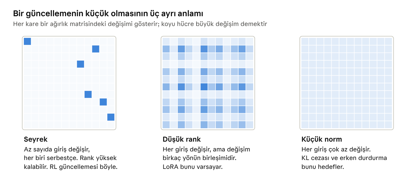
None of these implies the others. A matrix with only one modified row is both sparse and low-rank. A matrix with a modified diagonal is sparse but full-rank. Adding the same small number to every entry yields a rank-1 matrix that is not sparse at all. Mukherjee and colleagues’ observation lies precisely at this distinction: the RL update is sparse yet almost full-rank. LoRA’s premise therefore operates along the wrong axis for RL.
Behind all three criteria is a shared intuition: intrinsic dimension. Li and colleagues showed in 2018 that training a network in a randomly selected low-dimensional subspace can come surprisingly close to training it in the full space. Aghajanyan and colleagues extended this to pretrained language models in 2020, finding that pretraining lowers intrinsic dimension. LoRA is an engineering realization of that idea. The studies here develop its counterpart along the sparsity axis.
2.2 Post-training regimes
Everything done after pretraining is called post-training. The papers compare three regimes.
Supervised fine-tuning (SFT). Demonstrations are available, and cross-entropy training increases their probability. The data is independent of the model: it may or may not resemble what the model itself would generate.
RL with verifiable rewards (RLVR). The model generates its own answers to a question, a verifier rewards each answer, usually as correct or incorrect, and training increases the probability of higher-reward answers. The most common algorithm today is GRPO: it samples a group of answers to the same question and computes each answer’s advantage relative to the group mean. No separate value network is needed. Dr. GRPO, DAPO, and BNPO are variants differing in normalization and loss details.
A numerical example helps. Suppose the model generates 8 answers, of which 2 are correct. The group’s mean reward is 0.25. Correct answers have advantage +0.75; incorrect ones have advantage −0.25. The update increases the probability of the tokens making up correct answers with weight 0.75 and decreases that of incorrect answers with weight 0.25. Now consider the extremes: if all 8 answers are wrong, or all are right, every advantage is zero and so is the gradient. RL can learn only from questions the model sometimes gets right and sometimes wrong. It cannot teach an answer the model never produces. This simple observation contains the seed of the article’s conclusion: RL adjusts the frequency of an existing capability rather than constructing a new one.
On-policy distillation (OPD). The student generates its own answers; a stronger teacher assigns probabilities to those answers, and the student is moved toward the teacher. Unlike classical distillation, the data comes from the student itself rather than the teacher.
The main axis separating these regimes is whether they are on-policy. In RL and OPD, training data is sampled from the model’s current distribution. In SFT, data comes from outside; if it is close to the model’s distribution it is “near-policy,” and if distant it is “off-policy.” As Section 4 will show, this axis is the key to sparsity.
2.3 Anatomy of a transformer block
To follow the papers’ answers to “which weights,” we need to know the seven linear projections in a block. In the Llama and Qwen families, each block contains an attention layer and a SwiGLU MLP.
| Projection | Location | Function | Role |
|---|---|---|---|
| Q, K | Attention | Determine which positions to attend to | Reader |
| V | Attention | Determines what to retrieve from the attended position | Reader |
| O | Attention | Writes the retrieved information to the residual stream | Writer |
| Gate | MLP | Determines how much each intermediate neuron opens | Internal computation |
| Up | MLP | Computes the value carried by an intermediate neuron | Internal computation |
| Down | MLP | Writes intermediate neurons to the residual stream | Writer |
The SwiGLU MLP is:
Gate and up read the same input; their outputs are multiplied elementwise, and down writes the product back into the residual stream. Gate acts multiplicatively: if an intermediate neuron’s gate value is near zero, that neuron is silenced regardless of what up computes. This detail becomes decisive in Section 6.
The MLP dominates parameter count. In the LoRA placement paper’s breakdown for Qwen2.5, gate and up each contain 38.4% of LoRA-B parameters; Q, O, and down each contain 7.1%; K and V each contain 0.9%. Thus, a randomly chosen weight has about a three-in-four chance of belonging to gate or up.
2.4 LoRA and the B matrix
LoRA adds a low-rank correction alongside a frozen weight matrix W:
A is randomly initialized and B starts at zero, so the model initially matches the base model. A projects the input into an r-dimensional subspace; B writes from that subspace back into the output space. If A is frozen, each entry of B answers “how strongly should this random input direction connect to this output neuron?” The paper in Section 5 counts these entries individually.
2.5 Fisher information
Fisher information measures how much the model’s output distribution changes when a parameter is perturbed slightly. The full Fisher matrix is N × N and intractable; in practice only its diagonal is used. For parameter i:
Two details matter. First, y is sampled from the model itself; no labels, rewards, or teacher are needed. Fisher describes the model’s own behavior. Second, the derivative inside the brackets is the score, whose expectation is zero; Fisher is therefore its variance. If a parameter’s Fisher is small, its effect on log-probability is almost the same regardless of which answer the model produces.
A hand calculation makes this concrete. Suppose the model has three next-token candidates: tea with probability 0.6, coffee 0.3, and water 0.1. Consider four parameters, each affecting the logits differently. As we will see in Section 4.2, Fisher at one token position is the variance of a parameter’s logit sensitivities under the model’s own probabilities.
| Effect on logits when the parameter increases (tea, coffee, water) | Fisher | Interpretation |
|---|---|---|
| Increases all three (+1, +1, +1) | 0 | Differences do not change; probabilities stay the same |
| Increases tea and coffee (+1, +1, 0) | 0.09 | Only suppresses low-probability water |
| Increases coffee only (0, +1, 0) | 0.21 | Promotes the second candidate |
| Increases tea, decreases coffee (+1, −1, 0) | 0.81 | Changes the preference between two strong candidates |
All four parameters perturb logits by the same magnitude, yet their Fisher values range from zero to 0.81. The decisive issue is not a parameter’s strength but whether it distinguishes candidates the model takes seriously. According to Paper A, most parameters in a real model behave like the first two rows; this produces the sparsity under discussion.
Fisher is familiar in continual learning: Elastic Weight Consolidation (Kirkpatrick and colleagues, 2017) treats high-Fisher weights as important to an old task and penalizes their movement. Here the use is reversed: high-Fisher weights are precisely those the new task will also affect. We return to this tension in Section 10.
3. Roots: pruning research returns to fine-tuning
None of the tools used by these three papers is new. What is new is directing thirty years of pruning tools toward a different question: instead of “which weight can I remove,” ask “which weights are sufficient to change?” Seeing this family tree makes it easier to identify what is truly surprising in today’s results.
3.1 Importance scores: from 1989 to Wanda
The first question was always the same: how can I measure a weight’s importance without training?
Optimal Brain Damage (LeCun, Denker, and Solla, 1989) makes a second-order expansion of the loss around a weight and retains only the Hessian diagonal. The effect of deleting a weight is estimated by multiplying its squared value by the corresponding diagonal Hessian term. Since the expected Hessian for log-likelihood losses equals Fisher, this score is effectively diagonal Fisher times the squared weight. The object at the center of Section 4’s paper was already being used for the same purpose 37 years ago.
Optimal Brain Surgeon (Hassibi and Stork, 1993) drops the diagonal assumption, uses the inverse of the full Hessian, and compensates the remaining weights after deleting one.
Magnitude pruning (Han and colleagues, 2015) discards all this and deletes weights solely by small absolute value. It works surprisingly well and becomes the default for years.
SNIP (Lee and colleagues, 2018) moves scoring to initialization: one backward pass measures each connection’s sensitivity to the loss, and the sparse network trains from there. The procedure in Section 5—selecting entries with 50 initial backward passes—is a direct descendant.
Wanda (Sun and colleagues, 2023) is a pruning score for the LLM era: absolute weight value multiplied by the norm of its input activation. No gradients are required; a few calibration examples suffice. Deletion Tuning initializes its mask with this score.
3.2 Learning masks: training the selection rather than the weights
The second lineage starts from a more radical idea: leave the weights entirely untrained and learn only which ones remain.
The Lottery Ticket Hypothesis (Frankle and Carbin, 2018) proposed that a randomly initialized dense network contains a sparse subnetwork that, trained alone, can match the full network’s accuracy. Today’s finding that “RL trains a small subnetwork” says the same thing about pretrained models.
Supermasks (Zhou and colleagues, 2019) went a step further: learning only a mask over untouched random weights could achieve accuracy well above chance. Ramanujan and colleagues brought this to ImageNet scale the same year. Their message was that deletion is itself a form of learning.
Piggyback (Mallya and colleagues, 2018) is Deletion Tuning’s closest ancestor. A pretrained vision network is frozen, and a binary weight mask is learned for each new task. One backbone, one bit per weight per task. The goal was the same: multiple tasks without forgetting.
Masking language models (Zhao and colleagues, 2020) applied this idea to BERT-class models and obtained results comparable to fine-tuning, though by masking a substantial fraction of weights.
3.3 Sparse fine-tuning: training a small subset
The third lineage trains weights, but only a small fraction.
Diff pruning (Guo and colleagues, 2020) directly encourages a sparse task delta, approaching fine-tuning performance while storing about 0.5% of parameters per task.
FISH Mask (Sung and colleagues, 2021) selects high-Fisher parameters before training, fixes the mask, and trains only those parameters. This is the procedure in Section 4’s experiment. The difference is that in 2021 there was no theory explaining why it worked.
Movement pruning (Sanh and colleagues, 2020) considers movement direction during fine-tuning rather than magnitude: weights moving toward zero are pruned. It was among the first widely used scores to measure gradient-sign consistency across steps, anticipating the idea in Section 5.
3.4 The family tree
| 2026 study | Tool | Closest ancestor | What is new |
|---|---|---|---|
| Fisher perspective | Diagonal Fisher, fixed mask | OBD (1989), FISH Mask (2021) | A proof of why Fisher bounds gradients, with one explanation across regimes |
| LoRA placement | Gradient scoring at initialization | SNIP (2018), movement pruning (2020) | Showing that placement is largely irrelevant in SFT but decisive in RL |
| Deletion Tuning | Learned binary mask, Wanda initialization | Piggyback (2018), supermasks (2019) | Masking fewer than 0.05% of weights and matching FFT under RL |
| Weight-Space Programming | An LLM reading and writing weights | Manual circuit analysis, compiler-based weight generation (Tracr) | A general-purpose model doing the work instead of a human or compiler |
The tools are old, but three things are genuinely new. First, scale: Piggyback stored one bit per weight per task; Deletion Tuning compresses its mask to 0.03 bits per weight. Second, the distinction between regimes: earlier work lived in the SFT world, without recognizing that sparsity is strongest in on-policy training. Third, explanation: the first closed-form argument for why some weights receive no gradient.
4. Why sparse: the Fisher perspective
Zhang, Mukherjee, and Peng explain sparsity with one inequality: a parameter’s expected gradient is bounded by the square root of its diagonal Fisher. A low-Fisher parameter cannot receive a substantial gradient, regardless of the training signal.
4.1 The argument’s structure
The key observation is that expected gradients in all three regimes can be written in the same form. The model samples y from its own distribution, h_i is that sample’s score with respect to parameter i, and a(x,y) is a regime-specific effective signal:
Once in this form, the rest is a one-line Cauchy–Schwarz inequality:
The right-hand side separates into two factors, and that separation is the substance of the paper. The second depends only on the model and parameter; it knows nothing of the task, reward, or teacher. The first depends only on the training signal and is shared by all parameters. Thus, the answer to which parameters will receive gradients is already written in the model before training begins.
The effective signal in each regime is:
| Regime | Effective signal a | Signal scale | When small |
|---|---|---|---|
| On-policy RL | Reward minus the question’s mean reward | Conditional reward variance | Always bounded; at most 0.25 for binary rewards |
| OPD, policy-gradient form | Teacher score’s deviation from its mean | Conditional variance of teacher scores | When student and teacher are close |
| OPD, full-vocabulary form | Aggregate deviation of teacher/student probability ratios | Second moment of ratio deviations | When student and teacher are close |
| SFT | Data probability divided by model probability, minus one | Chi-squared distance between data and model | When data is close to the model’s distribution |
The SFT row deserves explanation because it is the least intuitive part. The SFT gradient is an expectation over the data distribution. To convert it into an expectation over the model’s distribution, multiply by the importance-sampling ratio w = data probability / model probability. Since the score has zero expectation, replacing w with w − 1 changes nothing. The second moment of w − 1 is, by definition, the chi-squared divergence between data and model. The closer the data resembles what the model would generate, the tighter the bound. As data becomes less familiar, chi-squared divergence grows, the bound loosens, and even low-Fisher parameters may receive gradients.
This explains the earlier empirical observation in one sentence: RL and OPD are always sparse because they are on-policy; SFT is sparse only with near-policy data. The paper does not say the bound “fails” for off-policy SFT, only that it becomes loose. That distinction matters.
4.2 Why Fisher is small: a token-level explanation
The inequality says “small Fisher implies a small gradient,” but not why most parameters have small Fisher. That is the paper’s second contribution.
Expanding the softmax derivative at one token position shows that a parameter’s score is the sampled token’s logit sensitivity to that parameter, minus the probability-weighted mean sensitivity of all tokens. The expected square, or token-level Fisher, is a variance:
Fisher is therefore the variance of logit sensitivities under the model’s own probabilities. It is small in two cases: either the parameter affects no logits, or it affects all likely tokens similarly. The second is more interesting. If the model is choosing between “tea” and “coffee” and a parameter pushes both logits upward together, changing it does not change their relative preference. The output distribution stays the same and Fisher is near zero. (This is the paper’s explanatory example, not a measured result.)
To test this, the authors compare actual token Fisher with the variance of the same sensitivities under a uniform distribution. A ratio below 1 means tokens the model considers likely respond more similarly than randomly selected tokens. The ratio is initially 0.16 and falls to 0.04 after 1,000 RL steps. In the lowest-Fisher parameter groups, it ranges from 0.03 to 0.11.
There are two interpretations. First, sparsity is a product of pretraining: as the model learns sharp, consistent predictions, most parameters settle into directions that do not change preferences. Second, RL reinforces this: the fall from 0.16 to 0.04 suggests increasingly decisive predictions and self-reinforcing sparsity.
4.3 Experiments
Setup. RL uses Qwen3-1.7B-Base with Dr. GRPO on SimpleRL-Zoo mathematics data, evaluated on MATH-500. There are 1,000 updates, learning rate 5e-7, 4 questions per update, 8 answers per question, and four seeds. Initial Fisher is estimated from 800 questions with one model answer each.
Does Fisher know where gradients will appear? Before training, the top 1% of coordinates by Fisher contains 47.40% of the top 1% by gradient magnitude. Random selection would yield 1%. For OPD, the same overlap is initially 35.66%, reaching 47.86% after 20 steps.
Training with a fixed Fisher mask. The central test is to select the top q% of parameters by initial Fisher, freeze the rest, and train only those selected.
| Fraction trained | Fisher mask | Random mask | Full-training improvement recovered |
|---|---|---|---|
| 0.05% | 49.65 | 23.21 | 79.98% |
| 0.1% | 51.41 | 23.90 | 85.21% |
| 0.5% | 54.00 | 26.42 | 92.87% |
| 1% | 55.03 | 31.07 | 95.90% |
| 5% | 56.01 | 47.59 | 98.82% |
MATH-500 accuracy. Initial accuracy is 22.65; full training reaches 56.41.
The random-mask column is the most striking. Training a random 0.05% of parameters moves the model from 22.65 to 23.21, effectively doing nothing. The same number selected by Fisher reaches 49.65. Sparsity does not mean any small subset suffices; a particular subset does.
OPD results point the same way but are noisy: evaluation uses 30 AIME24 questions, and 0.5% and 1% Fisher masks outperform full training on pass@8 (52.50 and 55.00 versus 47.50). With thirty questions, this amounts to two or three questions; it would be wrong to conclude that masking beats full training.
4.4 Critical reading
The paper is careful and keeps its claim narrow. Six points remain worth bearing in mind.
The bound is one-way. Small Fisher guarantees a small gradient; large Fisher does not guarantee a large gradient. The 47% overlap illustrates this: over half of high-Fisher parameters are not among those with the largest gradients. Fisher is an exclusion criterion rather than a sufficient selection criterion.
The expected gradient is not the actual update. The bound concerns a single step’s expected gradient at a fixed policy. The authors explicitly do not model optimizer dynamics, gradient noise, or learning-rate schedules. In our reading, Adam is the largest gap. Adam divides each parameter’s gradient by its own past magnitude; a small, consistent gradient can produce as large a step as a large, noisy one. Under Adam, what matters is the ratio of a gradient’s mean to its noise, not its magnitude. This is exactly what Section 5’s paper measures, making it the missing link between the papers.
One model, one scale. All experiments use the Qwen3-1.7B family. The finding is not replicated across families or scales.
No magnitude baseline. Fisher masks are compared only with random masks. Masks selected by weight magnitude, Wanda, or direct gradient magnitude are not tested. Section 5’s paper compares mean-gradient scoring with Fisher and finds very similar results, suggesting Fisher might not be special. We run the missing comparison at small scale in Section 8.3.
Where are the high-Fisher parameters? No layer- or module-level breakdown is given. The anatomical answer to “which weights” is absent; Section 5 fills that gap.
No demonstrated computational savings. Masked training uses dense computation: all gradients are calculated and those outside the mask discarded. The authors present Fisher selection as a test of their explanation rather than a proposed training method.
5. Which parameters: the placement problem in LoRA
Sehanobish and Lovering reduce the question to its simplest form: given a budget of k trainable parameters, does it matter which k you choose? Under RL the answer is “it determines everything”; under SFT, “almost not at all.” Gradient geometry explains the difference.
5.1 Experimental setup
The setup is deliberately constrained. Standard LoRA is attached to every linear layer in a block. A is randomly initialized and frozen; B starts at zero, and only k entries of B train. For Qwen2.5-1.5B, the B matrices contain about 20.6 million entries in total. Budgets range from 1,000 to 500,000, with the main results between 5,000 and 100,000: roughly one ten-thousandth to half a percent of B.
Why B alone? The paper also distributes the same budget across A and B and shows B-only training winning at every budget. With 1,600 parameters in Qwen2.5-1.5B, GSM8K accuracy is 61.2% when only B trains, versus 9.3% when both A and B train. There is a simple algebraic reason (our observation): when B is zero, the loss derivative with respect to A is also zero, because B annihilates A’s output. A entries cannot be scored initially, and their allocated budget stays inactive until B grows sufficiently.
5.2 Scoring procedure
Selection happens once, before training. At initialization, N forward-backward passes are run, and each B entry receives one of two scores:
The globally highest-scoring k entries are then selected across all modules and layers. The default is N = 50. N = 10 recovers over 90% of the reference circuit obtained with 100 passes; N = 50 recovers about 98%. (“Circuit” is the paper’s name for the selected entries.) This takes under 10 seconds on one GPU and costs 0.49% of SFT training FLOPs or 0.18% of GRPO FLOPs.
The relationship between the scores is instructive. The second moment equals the squared mean plus variance. Thus F̂ identifies entries with large gradients regardless of sign consistency. Ŝ rewards only entries whose gradients point the same way across examples; an entry whose sign keeps changing averages toward zero. There is no separate sign-consistency threshold: the absolute mean performs that role automatically. Their similar empirical results suggest that under RL, large-gradient and consistent-gradient entries largely coincide.
A terminology warning: F̂ here belongs to the same family as Fisher in Section 4, but is not the same object. Section 4 samples from the model’s distribution without labels. Here the appendix says circuit discovery uses cross-entropy loss, so the score sees task data. The first measures the model; the second measures the model-task combination.
5.3 Main result: regime changes everything
Random placement does not learn under GRPO. Training uses GRPO on MATH, with evaluation on GSM8K and MATH-500:
| Model, evaluation | Base | Random | Ŝ | F̂ | Full LoRA |
|---|---|---|---|---|---|
| Qwen2.5-1.5B, GSM8K | 9.5 | 9.8 | 64.2 | 63.2 | 62.8 |
| Qwen2.5-3B, GSM8K | 62.1 | 62.3 | 70.6 | 73.6 | 71.9 |
| Qwen2.5-7B, GSM8K | 79.3 | 79.6 | 85.2 | 86.3 | 87.6 |
| Qwen2.5-1.5B, MATH-500 | 17.4 | 18.8 | 43.6 | 42.2 | 41.4 |
| Qwen2.5-3B, MATH-500 | 50.6 | 51.0 | 60.4 | 63.2 | 62.6 |
| Qwen2.5-7B, MATH-500 | 53.6 | 55.2 | 74.8 | 76.0 | 74.6 |
| Llama-3.2-3B-Inst, GSM8K | 70.4 | 67.9 | 73.9 | 72.6 | 74.7 |
| Llama-3.1-8B-Inst, GSM8K | 82.9 | 83.4 | 86.2 | 85.9 | 86.4 |
| Llama-3.2-3B-Inst, MATH-500 | 43.6 | 50.2 | 50.8 | 51.0 | 50.8 |
| Llama-3.1-8B-Inst, MATH-500 | 50.4 | 53.2 | 54.6 | 55.8 | 56.6 |
Accuracy (%). Budgets are 10,000 or 50,000 entries.
For base models the contrast is sharp: random selection reproduces the base column, whereas informed placement matches full LoRA and sometimes exceeds it. Random placement’s failure is not a hyperparameter accident: sweeping LoRA alpha from 32 to 4,096 and budgets from 1,000 to 10,000 leaves Qwen2.5-1.5B between 9.3% and 9.8% on GSM8K.
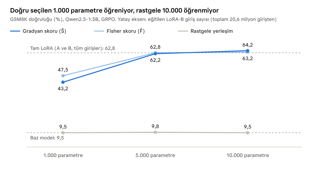
Informed placement catches up with full LoRA at 5,000 entries; random placement never leaves the base-model line.
The gap shrinks for instruct models. On Llama-3.2-3B-Instruct’s MATH-500 row, random scores 50.2 versus 50.8 and 51.0 for informed selection. We return to this in Section 5.6 because it determines the scope of the paper’s title claim.
Placement is largely irrelevant under SFT. SFT on Alpaca, averaged over seven benchmarks:
| Model | Base | Random | Ŝ | F̂ | Full LoRA |
|---|---|---|---|---|---|
| Qwen2.5-1.5B | 53.0 | 61.6 | 61.9 | 62.1 | 62.4 |
| Qwen2.5-3B | 65.6 | 65.8 | 66.2 | 66.0 | 66.7 |
| Qwen2.5-7B | 70.9 | 71.1 | 71.4 | 71.5 | 71.5 |
| Llama-3.2-3B-Inst | 62.3 | 62.9 | 63.8 | 63.7 | 63.9 |
| Llama-3.1-8B-Inst | 68.7 | 69.1 | 69.6 | 69.7 | 69.9 |
The random/informed gap is below one point in every row. But the table hides two things. First, in four of five rows full LoRA itself improves on the base model by only one or two points; placement being unimportant is unsurprising when there is little to learn. Second, a harder SFT task changes the picture: Qwen2.5-7B-Instruct trained on Bespoke-Stratos and evaluated on GPQA Diamond scores 41.1 with 5,000 random entries, 43.3 with Ŝ, and 50.7 with full LoRA. All sparse-B methods lag full LoRA, while F̂ scores 31.1, essentially the base level of 31.6. The paper does not explain this result.
5.4 Mechanism: gradient geometry
The main contribution is the explanation rather than the result table. Three measurements distinguish the regimes:
| Model | Effective rank (SFT / GRPO) | Cross-step cosine (SFT / GRPO) | Accumulation efficiency (SFT / GRPO) |
|---|---|---|---|
| Qwen2.5-1.5B | 2.6 / 21.8 | 0.76 / 0.04 | 0.90 / 0.28 |
| Qwen2.5-3B | 5.8 / 7.7 | 0.61 / −0.03 | 0.81 / 0.22 |
| Qwen2.5-7B | 2.0 / 8.8 | 0.85 / −0.03 | 0.93 / 0.18 |
These columns tell the same story from three perspectives.
Effective rank counts the independent directions in a single step’s gradient: two or three for SFT, eight to twenty-two for GRPO.
Cross-step cosine measures whether consecutive gradients point the same way. SFT ranges from 0.6 to 0.85: each step repeats the previous one. GRPO is near zero: each step is orthogonal to the last.
Accumulation efficiency divides the length of the vector sum of steps by the sum of step lengths. For SFT, nine out of every ten units walked become progress. For GRPO, four-fifths cancel out.
The connection to placement is as follows. Selecting k random entries projects the gradient onto a random k-dimensional subspace. In SFT, the gradient stays similar across steps, so its projection does too; however small, the push keeps pointing the same way and accumulates. In GRPO, most of the gradient is noise that cancels across steps. Persistent signal lives in very few sign-consistent entries. A random subset contains almost none, leaving pure noise.
Think of a walk of 2,000 unit-length steps; Paper B’s GRPO training also lasts 2,000 steps. If every step points the same way, you advance 2,000 units. If each points randomly, expected displacement is on the order of the square root of the step count: about 45 units. The same effort, forty-four times less distance. SFT resembles the first walk; GRPO the second. What produces progress in GRPO is the small component pointing the same way at each step, and it occupies few coordinates.
Two numbers reinforce this picture. The highest-scoring 0.05% of B entries carry 8–15% of gradient energy, 160–300 times random expectation. Selected entries move 1.4–2.1 times as far as random entries during GRPO training. Under SFT the reverse holds: selected entries move less, only 0.24–0.41 times as far. This suggests entries with large initial SFT gradients saturate quickly and the remaining work happens elsewhere. An initial SFT score does not predict the final update well.
This connects to Section 4. The Fisher bound identifies where the expected gradient will vanish. This paper measures noise around that expectation and shows that in RL it overwhelms the signal almost everywhere. Together they give a fuller picture: in on-policy training, signal occupies few coordinates (Fisher), while everything outside them cancels across steps (cosine).
5.5 Anatomy of the circuit
Where in the block are selected entries? Although gate and up dominate parameter count, selection does not concentrate there.
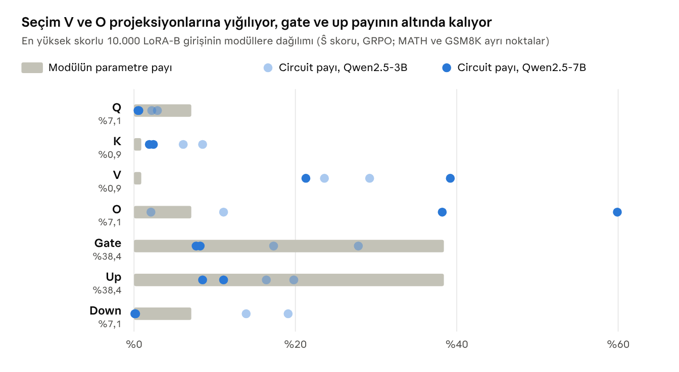
A gray bar shows the share a module would receive under random selection; points show its actual share. A point to the right of its bar means overrepresentation, to the left underrepresentation.
Three regularities stand out.
V is overrepresented in every setting. V contains 0.9% of parameters but receives 21–39% of the circuit: 23–43 times its share.
O dominates in the larger model. O receives 2–11% in 3B but 38–60% in 7B. Conversely, down receives 14–19% in 3B and falls almost to zero in 7B. The abstract says “V, O, and down,” but the table varies by model; only V is stable.
Gate and up are underselected. Together they contain 77% of parameters but receive 37–44% of the circuit in 3B and 16–19% in 7B. The appendix notes that their gradient signs are as consistent as V and O, so consistency is necessary but insufficient. The authors explain that gate and up affect the residual stream indirectly, through the MLP’s internal computation.
Concentration by depth is sharper still. The first five layers (0–4) receive 71.7% of the budget in Qwen-3B, 98.9% in Qwen-7B, 97.4% in Llama-3B, and 96.8% in Llama-8B. Qwen-7B-Instruct is the exception: early layers receive only 18%, and the budget shifts to middle and late layers.
An ablation supports causality: zeroing the highest-scoring entries of a fully trained LoRA reduces accuracy much faster than zeroing equally many random entries. For Qwen-7B on MATH, this removes 12.2 points of LoRA’s 21.6-point gain.
5.6 Critical reading
The claim is specific to base models. The appendix is explicit: instruct models produce diffuse gradients in both regimes, and the SFT/GRPO contrast disappears. Since many models trained with RL in practice are instruct models, this is the paper’s most important limitation. Why it happens is unexplained. One hypothesis is that instruction fine-tuning already exploits and saturates the “easy” early-layer circuit; Qwen-7B-Instruct’s shift toward later layers fits that account.
Early-layer concentration may be a scale artifact. Selection is global: all layers’ entries compete in one pool using raw gradient magnitude. If early layers systematically have larger gradient norms, global ranking favors them. We found no comparison with layer-normalized selection. A concentration of 98.9% could be functional or a normalization artifact. Section 11 proposes an experiment to distinguish these possibilities.
“Which entry” is relative to a random basis. B entries depend on the frozen random A. A small perturbation to A (ε = 0.1) preserves 92–94% of the top 10,000 entries; a completely different A (ε = 1.0) reduces overlap to 42–54%. Yet module- and layer-level distributions vary by at most 3 points over eight A seeds. The stable objects are therefore modules and layers, not individual entries.
Scope. Only mathematical reasoning is tested, not code, dialogue, or open-ended tasks. The largest model is 8B. The authors also note that realizing an O(k) cost advantage requires custom sparse kernels; the current implementation still computes all gradients.
Internal inconsistencies. Some main-text numbers—“nearly rank-1” and cosine 0.87 for SFT, “rank-24” and cosine 0.08 for GRPO—do not exactly match the table above. LoRA rank also differs between the text and hyperparameter table. These discrepancies do not change the direction of the result, but table values are safer to cite. This assessment used extracted text and should be checked against the original PDF.
6. How little: Deletion Tuning
Lu and colleagues (NeurIPS 2026) take sparsity to its extreme: no weight receives a new nonzero value; some are simply zeroed. In models of 7B and above, deleting fewer than 0.05% of weights matches full fine-tuning under GRPO while preserving almost all previous capabilities.
6.1 Mechanics
Parameterization. Only MLP gate projections are targeted. Each gate weight receives a logit G. The weight stays frozen; only G trains. During training, the effective weight is computed with a soft mask:
For GRPO, sharpness α rises linearly from 1,000 to 10,000 over training. Evaluation and RL sampling use a hard mask: keep the weight if G is positive, otherwise delete it. The paper reports at most a 0.08-point difference between soft and hard masks; at such high α the sigmoid is already nearly a step function. No straight-through estimator is used; gradients flow through the soft mask.
Initialization. Logits are initialized from Wanda scores rather than randomly. Important weights receive logits drawn around +0.03, less important ones around −0.03, with standard deviation 0.012. Training thus begins with about 0.18% of gate weights already deleted. Its starting point is a lightly pruned base model, not the base model itself.
No sparsity target. The deletion count is not fixed in advance; it emerges during training. GRPO and SFT include a small regularization term tied to masked weight norms (λ = 1e-5; the authors say it gently favors preserving large weights), whereas OPD does not.
Why gate? In SwiGLU, gate multiplicatively determines each intermediate neuron’s signal to down. Deleting a gate weight removes one residual-stream dimension’s contribution to a neuron’s activation decision. What the neuron computes (up) and where it writes (down) stay unchanged; only when it activates changes. In the MoE model, gates inside all 128 experts are masked, while the router remains unchanged.
Storage. The mask is bit-packed and compressed with zstd to about 0.03 bits per masked weight. Deletions are so sparse that the mask is almost all ones and compresses very well.
A rough calculation helps (ours, not the paper’s). Llama-3 8B has a 4,096 × 14,336 gate matrix in each of 32 layers: about 1.88 billion weights, close to a quarter of the model. Taking 0.18% of that gives roughly 0.04% of all weights. The paper’s final figure is below 0.05% in every GRPO run. They are of the same order. If this calculation is right, training changes the mask’s location more than its size: some initially deleted “unimportant” weights return, while task-specific ones are deleted. Table 7 supports this reading: Llama-1B’s deleted fraction is 0.0342% at the first recorded checkpoint and 0.0347% at the end. The net count barely changes. Mask-entry turnover is not reported, so these figures cannot distinguish learning by swaps from learning completed before the first checkpoint.
6.2 Is the mask actually learned?
Wanda initialization raises an obvious objection: perhaps Wanda does the work rather than training. The paper tests this directly. The best Wanda-only mask stays within 2.4 points of the base model, while training from the same initialization yields gains of up to 53.2 points. Pruning scores provide a starting point; selection learned from the RL signal produces the capability.
6.3 Results
GRPO. Llama models train and evaluate on GSM8K (in-distribution). Qwen models train on SimpleRL-Zoo mathematics data and evaluate on the average of six benchmarks (out-of-distribution).
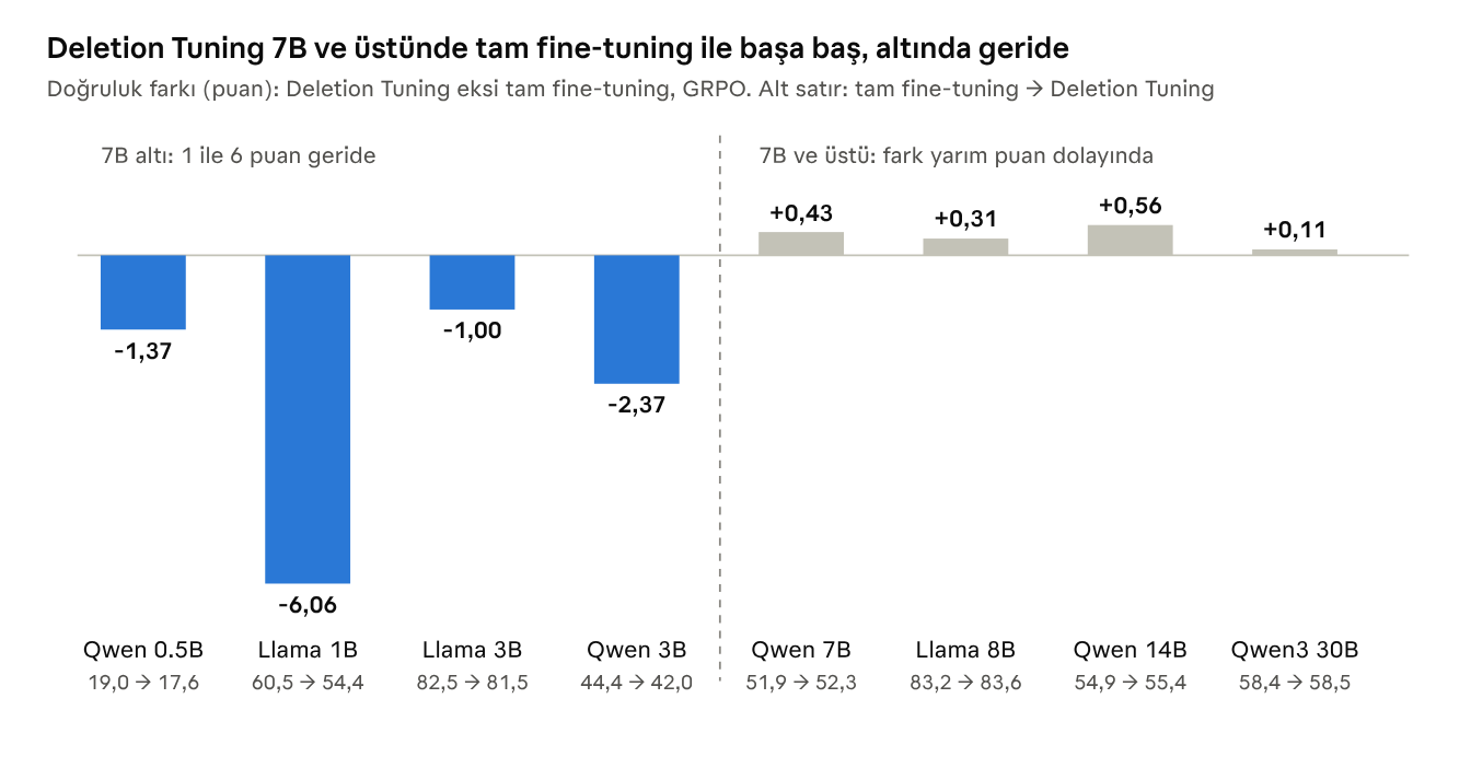
The chart is clear: the gap closes with scale and changes sign from 7B onward. Between 0.5B and 3B, Deletion Tuning trails by 1–6 points; at 7B, 8B, 14B, and 30B it leads by 0.1–0.6 points. The latter differences are at noise level, so the right reading is “equal,” but the deficit in smaller models is systematic.
The other two baselines in the table matter too. Rank-1 LoRA and MTH (Multiple Ticket Hypothesis, a baseline training a random 0.05% of all parameters) score 83.38 and 83.07 on Llama-8B, and 52.13 and 51.24 on Qwen-7B. In large models all four methods are thus within about half a point. Accuracy does not distinguish Deletion Tuning; storage and forgetting do.
Size.
| Model | Full fine-tuning checkpoint | Deletion Tuning mask | Ratio |
|---|---|---|---|
| Llama 8B | 30,633 MB | 8.4 MB | about 3,600× |
| Qwen 7B | 29,051 MB | 6.9 MB | about 4,200× |
| Qwen 14B | 56,343 MB | 11.4 MB | about 4,900× |
| Qwen3 30B (MoE) | 116,471 MB | 29.6 MB | about 3,900× |
Pass@k: the capability was already there. This is, in our view, the paper’s most instructive but least discussed table. Base Llama-8B scores 53.20% on GSM8K in one attempt, but 95.29% when any of 128 attempts may be correct. The base model can solve almost every question; it simply does not produce the correct answer every time. After Deletion Tuning, single-attempt accuracy rises to 81.75%, and 128-attempt accuracy to 99.62%. What changes is how often the model does what it can do, rather than what it can do. This is the most direct evidence for the article’s thesis: RL post-training concentrates probability mass on existing correct behavior.
SFT and on-policy distillation. The picture is more mixed here.
| Regime, model, task | Full fine-tuning | Deletion Tuning |
|---|---|---|
| SFT, Llama 3B, MMLU-Pro (14 subjects) | 21.19 | 22.28 |
| SFT, Llama 1B, BBEH (23 subtasks) | 8.35 | 5.65 |
| OPD, Qwen 7B, ToolAlpaca | 68.04 | 69.07 |
| OPD, Qwen 7B, Science | 71.20 | 70.61 |
Distillation mask sizes are notable: 27.1 and 47.1 MB, versus 6.9 MB for the same Qwen-7B under GRPO. Distillation requires four to seven times as much deletion as RL. In our reading, this is a side finding consistent with Section 4’s prediction: as the training signal moves away from the model’s distribution, the set of weights needing modification grows.
6.4 Forgetting
The paper measures forgetting in two ways: divergence of the trained output distribution from the base (forward KL), and accuracy on six previous tasks: HellaSwag, MMLU, TruthfulQA, WinoGrande, IFEval, and HumanEval.
| Method | Forward KL at training end | Previous-task accuracy relative to base |
|---|---|---|
| Full fine-tuning | 1.0 (1B) to 1.5 (8B) | 1.3–3.1 points lower |
| LoRA r=1 and MTH (random sparse) | 0.4–1.3 | Up to 5.4 points lower |
| Deletion Tuning | 0.05 or less | Within one point |
The KL gap is twenty- to thirtyfold, much greater than the half-point accuracy differences and the paper’s main selling point. Interestingly, rank-1 LoRA forgets more than FFT: training few parameters does not by itself reduce forgetting; the form of the change matters too.
One limitation must be explicit: forgetting is measured after training a single task. No actual continual-learning experiment with sequential tasks is run; the authors leave that for future work.
6.5 Update geometry
The paper compares deltas from four methods using three measures. They are standard tools in weight-space analysis and deserve individual explanation.
Stable rank. The squared Frobenius norm divided by the squared spectral norm:
It is a noise-robust version of rank, indicating how many singular directions carry energy. For rank-1 LoRA it is, by construction, between 1 and 2. For random sparse MTH it is 410–650; for Deletion Tuning, 66–93. The deletion mask is therefore not low-rank, but neither is it as diffuse as a random sparse update: it occupies a structured region between them.
Spectrum drift. This measures changes in a weight matrix’s singular values after training. Deletion Tuning stays within 1.4× FFT’s drift. Rank-1 LoRA reaches up to 84× FFT on Llama-8B. Confining an update to one direction disproportionately inflates its singular value, potentially explaining LoRA’s greater forgetting.
Principal-weight overlap. This measures how much an update overlaps weights contributing most to the matrix’s leading singular directions; random expectation is 0.5. Deletion Tuning scores 0.43–0.46 and FFT 0.41–0.46, both below random. LoRA scores 0.48–0.50 and MTH 0.50. Drawing on Zhu and colleagues’ “The Path Not Taken: RLVR Learns Off the Principals” (NeurIPS 2026), the authors interpret below-random overlap and low spectrum drift as an RL signature: RL avoids principal directions and works on secondary weights.
All three measures agree: among the four methods, Deletion Tuning is geometrically closest to FFT. Measurements use two recorded checkpoints: Llama-8B at step 348 and Qwen-7B at step 100.
6.6 Why is deletion enough?
The paper offers no theoretical answer. Three possible explanations follow; all are our interpretations.
Combinatorial richness. Each entry in a deletion update is either zero or the negative of the existing weight; magnitude cannot be chosen. This seems restrictive, but the number of possible subsets is astronomical. A neuron’s preactivation sums thousands of terms; removing the right subset can move the sum toward almost any desired value. Theoretical lottery-ticket research proved precisely this: Malach and colleagues showed that a sufficiently wide random network can approximate any target network through pruning alone. A pretrained LLM is a much richer starting point than a random network.
RL already wants suppression. Pass@k shows correct behavior is already present. The task is to reduce the probability of paths producing wrong answers, inherently a subtractive operation. We would not expect the same method to work as well when new knowledge must be taught; the 1B BBEH result weakly points that way.
Redundancy grows with scale. The deficit in smaller models fits a lack of spare capacity to delete. In a 1B model each weight carries more work, and deleting one damages something else.
6.7 Critical reading
Critical ablations are missing. Other projections—Q, K, V, O, up, down—are not tested. Nor is freely training the same number of weights instead of deleting them. We cannot tell which of the title’s two choices, deletion or gate, does the work. Section 5 suggests gate may not be the most efficient target; we return to this tension in Section 9.
The random baseline is unexpectedly strong. MTH trains a random 0.05% of parameters and scores 51.24 on base Qwen-7B, versus 51.89 for FFT. This seems directly at odds with A and B’s finding that random sparse selection does not learn under RL. C does not address this contradiction. Section 9.3 discusses it in detail, because it appears only when the three papers are read together.
The saturated-sigmoid question. Logits start around 0.03 and α is at least 1,000. Their product is around 30, where sigmoid is nearly saturated and its derivative about 1e-13. In practice, gradients can flow only to weights with logits extremely close to zero. The paper does not discuss this. Our unverified interpretation is that initial Gaussian noise implicitly defines a candidate set, and training can move only near-threshold logits. If so, Wanda initialization and noise width may matter more than the hyperparameter table suggests. Table 7’s stable deletion rate fits this reading.
Training is not cheap. The method is parameter-efficient in storage, not training. A logit and optimizer state are maintained for every gate weight: about 1.9 billion trainable parameters in an 8B model. The authors say memory use is below FFT but above LoRA and suggest restricting logits to a candidate set. No runtime or FLOP comparison is supplied. The scores in Sections 4 and 5 could produce precisely such a candidate set.
Small models. The abstract’s “matches full fine-tuning” claim does not hold below 7B. For someone working with small language models, this is the paper’s most important footnote.
The baselines are fair. A credit to the paper: FFT learning rates and KL coefficients are swept, and no setting beats Deletion Tuning. Its own hyperparameter sensitivity is also low: deviations from the best setting remain within 1.6 points on Llama-8B and 3.2 on Qwen-7B.
7. The gradient-free route: Weight-Space Programming
Takehi, Teoh, Zhang, and Khattab (MIT CSAIL, 2 November 2026) question the preceding sections’ shared assumption: are gradients necessary to find which weights should change? They present eight cases in which a strong language model directly reads and writes weights. In the authors’ own terms, these are “sparks”: early evidence, not a finished method.
The evidential status differs from the previous three sections. The source is a blog post rather than a peer-reviewed paper, and the results are individual cases rather than experiments with baselines. On the other hand, all experiment logs are public, and the most striking result—the Qwen edit—has been independently reconstructed and evaluated.
7.1 The idea
Weights have traditionally been produced in three ways: optimization through gradient descent, other networks trained to generate weights, or compilation from a formal program. A familiar example of the last is Tracr, which compiles a RASP program into transformer weights. Weight-Space Programming proposes a fourth route: a reasoning, general-purpose model writes them.
The background is this: language models have recently optimized text artifacts of all kinds—prompts, agent harnesses, training code. One justification was the lack of a principled gradient-like way to hill-climb on text. Weights already had gradients, so writing them through reasoning was not explored. The post argues that this boundary is arbitrary.
All experiments use a model the authors call Astra. Small networks’ weights fit directly in context. For larger networks, the model inspects weights by running code in a sandbox, with a limited forward-pass budget in some experiments.
7.2 Eight experiments
| No. | Type | Network | Task | Result |
|---|---|---|---|---|
| 1 | Read | 4 PPO agents, same architecture, 17,253 weights | Identify the game from raw weights | 4/4 correct, no tools |
| 2 | Read | 3 diffusion models, 23,824 weights | Identify the generated shape without a forward pass | 3/3 correct |
| 3 | Read | 3 character-level transformers, 7.2M parameters, input/output layers removed | Identify training language and induction heads | 3/3 languages; all induction heads found, no false positives |
| 7 | Read | Gemma 3 270M, honest and sycophantic copies | Identify the sycophantic model | Fails in 4 weight-only attempts; 3/3 with attention patterns |
| 4 | Write | A failing PPO controller in Kinetix | Repair a policy trapped in a local minimum | 3.5% of weights changed; success from 0/256 to 1,024/1,024 |
| 5 | Write | Blank MinAtar networks | Write weights from scratch without data or gradients | Beats 100M-step PPO in all three games |
| 6 | Write | 1.48M-parameter network for 9×9 Go | Write a Go network without training or search | With 50 forward passes, beats an equally sized PPO network trained on 20M games |
| 8 | Write | Qwen3.5-0.8B | Locate and fix a known bug in the weights | 0.016% of weights changed; MATH-500 from 7.9% to 48.1% |
7.3 Reading: inferring behavior from weights
The methods are more interesting than the outcomes. In Experiment 1, the model infers the game from the input channels emphasized by the first layer: a game agent’s first layer maps which parts of observation space matter for decisions. In Experiment 2, it draws shape outlines even though the diffusion models generate filled shapes. The authors interpret this as evidence that it analyzes weight geometry rather than computing the output.
Experiment 3 is hardest. Removing input and output layers removes the vocabulary identifying which weights correspond to which characters; only internal computation remains. The model still identifies the training language. It diagnoses romanized Japanese from a restricted character set with no q, l, v, or x. Finding every induction head—attention heads that copy—with no false positives suggests that a manual mechanistic-interpretability analysis can be automated.
Experiment 7 marks the boundary and is the post’s most candid part. The model fails in all four weight-only attempts to identify sycophancy, the tendency to flatter or agree with the user. Given attention patterns on its own generated text, it succeeds on all three pairs: in the sycophantic copy, head 10.2 attends to the user’s suggested answer rather than numbers in the question. Structural features such as game, language, and head can be read from weights; subtle behavioral differences require activation space. Section 2.1’s distinction becomes concrete here.
7.4 Writing: constructing and repairing weights directly
Networks written from scratch. In Experiment 5, the model writes weights for three MinAtar games.
| Game | Handwritten network | PPO, 100M steps | PPO, 500M steps |
|---|---|---|---|
| Breakout | 517.4 | 15.8 | 25.3 |
| Seaquest | 53.1 | 5.6 | 88.9 |
| Asterix | 53.2 | 25.8 | 55.2 |
Breakout seems an outlier, but the explanation is simple: the model writes a first layer that predicts where the ball will land and a second that moves the paddle there. This is a closed-form solution. PPO does not discover it in 500 million steps. Seaquest and Asterix lack such clean solutions, so longer-trained PPO wins or matches it. The generalization is that explicit task algorithms can make weight writing far outperform optimization; without one, optimization remains better.
The Go experiment scales the same idea. Rather than write 1.48 million parameters individually—243 inputs, six 512-unit layers, 82 outputs—the model writes a 336-line Python program generating them. Its layered logic counts liberties, captures stones, and evaluates group safety. The version written without any forward passes beats two smaller PPO networks in over half the games. The important scaling strategy is generating weight-producing code rather than writing weights directly, escaping the context-window limit.
Repair. In Experiment 4, a PPO policy cannot drive a car up a ramp to its target, failing in all 256 attempts. The model explains the failure and makes one edit: a small bypass reading position and velocity that switches itself off after the car crosses a particular strip. It changes 3.5% of weights, succeeding in all 1,024 test episodes. Where gradient descent cannot escape a local minimum, an editor understanding the problem escapes in one move.
7.5 The Qwen case: one direction, 130,000 weights
Experiment 8 is most directly relevant here because it involves a real language model.
Qwen3.5-0.8B has a known flaw documented in its model card: looping during long generations. In the base model, 93% of MATH-500 answers hit the 32,768-token limit; even when the model knows the answer, it exhausts the budget before saying it. Astra traces this to one direction written into the residual stream by MLPs in layers 15 and 19 and removes that direction from 64 output columns in each layer. The edit changes 131,072 weights: two layers, 64 columns each, 1,024 entries per column—0.016% of the model.
| Measurement | Before | After |
|---|---|---|
| MATH-500 | 7.9% | 48.1% |
| GSM8K | 13.8% | 67.1% |
| IFEval | 21.0% | 62.3% |
| MATH-500 answers hitting the token limit | 93% | 33% |
These results require a budget of 50 forward passes. With 10 or 25, gains remain small and looping largely persists. This combines weight analysis with a few experiments rather than pure weight reading.
Correctly classifying the edit matters. The operation is not new: identifying a residual-stream direction and removing it from weights is familiar from refusal-direction work (Arditi and colleagues, 2024) and rank-1 model editing (Meng and colleagues, 2022). What is new is a model performing the diagnosis and surgery instead of a human researcher. Geometrically it also differs from Section 6: Deletion Tuning performs sparse, high-rank deletion; this is a dense, low-rank subtraction, rank-1 per layer. Both are subtractive and touch less than 0.05% of the model, but occupy different corners of Section 2.1’s three “smallness” axes.
7.6 The negative result and main lesson
The same approach brings no improvement to Gemma 3 270M. It rarely loops, and its edited MATH-500 scores stay within about one point of the 6.8% baseline. The authors’ conclusion is the post’s key sentence: editing weights can remove a barrier hiding a capability, but cannot add a capability the model lacks.
This says the same thing as Section 6’s pass@k table. Llama-8B could solve 95% of questions in 128 attempts; RL increased the frequency of correct answers. Qwen3.5-0.8B knew the mathematics; looping prevented it from expressing it. In both cases a small weight change produced a large score change by exposing an existing capability rather than building one.
7.7 Critical reading
No baselines. Natural comparisons are missing for the Qwen edit: could repetition penalties achieve the same gain? How quickly could a human identify the same direction through activation differences? The authors acknowledge dependence on particular sampling settings and benchmark protocols.
Selected cases. We do not know how many attempts produced the eight cases. The authors say a standard benchmark and evaluation harness is in progress but unfinished. Until then, these are existence proofs.
Scale. The largest complete read is 7.2 million parameters; work on the 0.8-billion-parameter model traces one known bug. Finding an unknown problem directly from the weights of a billion-parameter model remains undemonstrated. Context length and tool inefficiency are limitations the authors themselves identify.
The model’s own claims. The authors say Astra’s self-reported minor improvements are not treated as evidence. This is methodologically important: a weight-editing agent saying “fixed it” cannot replace independent measurement.
8. Our verification: testing the claims in a small model
We tested the three papers’ main claims from scratch in a 74,624-parameter model. Four of eight claims held in the same direction and four did not. One test produced a result absent from the papers: a Fisher-selected mask performs worse than a random mask when teaching the model something new.
This section is not a replication. A claim holding in a toy model neither proves it for real models nor, if it fails, refutes it. The aim is to distinguish mathematical necessities from empirical properties of real language models. A small model makes this possible because every expectation can be calculated exactly without sampling.
8.1 Setup
Model. 200 contexts, each with a 32-dimensional embedding; one 128-neuron tanh hidden layer; 500 output tokens. Total: 74,624 parameters—8.6% embedding, 5.5% input projection, and 85.8% output projection.
Language. Contexts are divided into 20 clusters. Each has five plausible continuations with probabilities 0.50, 0.25, 0.12, 0.08, and 0.05; contexts in the same cluster share a token pool. Half the vocabulary is plausible in no context, so the model never learns to produce those tokens. Pretraining fits this distribution to KL 0.0006.
Tasks. Two tasks represent two types of post-training.
Preference shifting: produce the second-most likely token rather than the most likely one in each context. Initial success is 0.25. The answer already exists in the model’s distribution; only probability mass must shift. This task trains with both RL—16 contexts, 8 samples per context, binary rewards, group-mean baseline—and SFT using the target token as label.
New token: produce a token never previously generated in each context. Initial success is 0.00. This adds a behavior the model lacks, is inherently off-policy, and can train only through SFT.
Masks. Four selection methods are compared at equal budgets: Fisher (exact diagonal Fisher from the model’s own samples), task gradient (absolute initial expected task gradient), weight magnitude, and random. The second and third are baselines Paper A did not compare.
Measurements. Success is mean target-token probability on training contexts. Collateral damage is KL drift from the initial output distribution on 48 contexts in four clusters never used in training, serving as a proxy for forgetting. Training uses Adam, learning rate 3e-3, 1,500 steps, and three seeds.
8.2 Test 1: does the Fisher bound hold, and how tight is it?
We calculate Paper A’s inequality exactly for nine training signals at each of 74,624 coordinates. There are zero violations, as expected from a theorem. Tightness is more interesting: actual gradient divided by the bound is 0.21 at the best coordinate and around one ten-thousandth at the median. The bound is correct but loose by four orders of magnitude at most coordinates. Fisher guarantees a small gradient without predicting how small it will be.
The central question is whether Fisher locates the gradient. Using Paper A’s metric, what fraction of the top 1% by gradient magnitude appears in the top 1% by Fisher?
| Training signal | Signal scale E[a²] | Top-1% Fisher hit rate |
|---|---|---|
| RL, on-policy | 0.19 | 58% |
| SFT, sharpened model distribution | 0.07 | 55% |
| SFT, target = most likely token | 1.0 | 67% |
| SFT, target = second-most likely token | 3.0 | 58% |
| SFT, target = fifth-most likely token | 19 | 24% |
| SFT, target = twentieth-most likely token | 150,000 | 19% |
| SFT, target = hundredth-most likely token | 470,000 | 21% |
| SFT, target = never-generated token | 500,000 | 14% |
Random expectation is 1%. Paper A measures 47% on Qwen3-1.7B.
This cleanly supports Paper A’s central claim. When the training signal is close to the model’s distribution (the first four rows), Fisher finds over half the highest-gradient coordinates. Once the target leaves the model’s five plausible tokens, hit rate falls to about a third and signal scale grows by five orders of magnitude. The chi-squared term is the numerical expression of the on-policy/off-policy difference rather than merely an abstract factor.
Why does hit rate fall? Fisher for a token’s output column is proportional to that token’s probability. If the model never produces a token, the weights that must change to produce it have near-zero Fisher. Fisher measures what the model currently does; it cannot know what it ought to do.
8.3 Test 2: which mask works on an on-policy task?
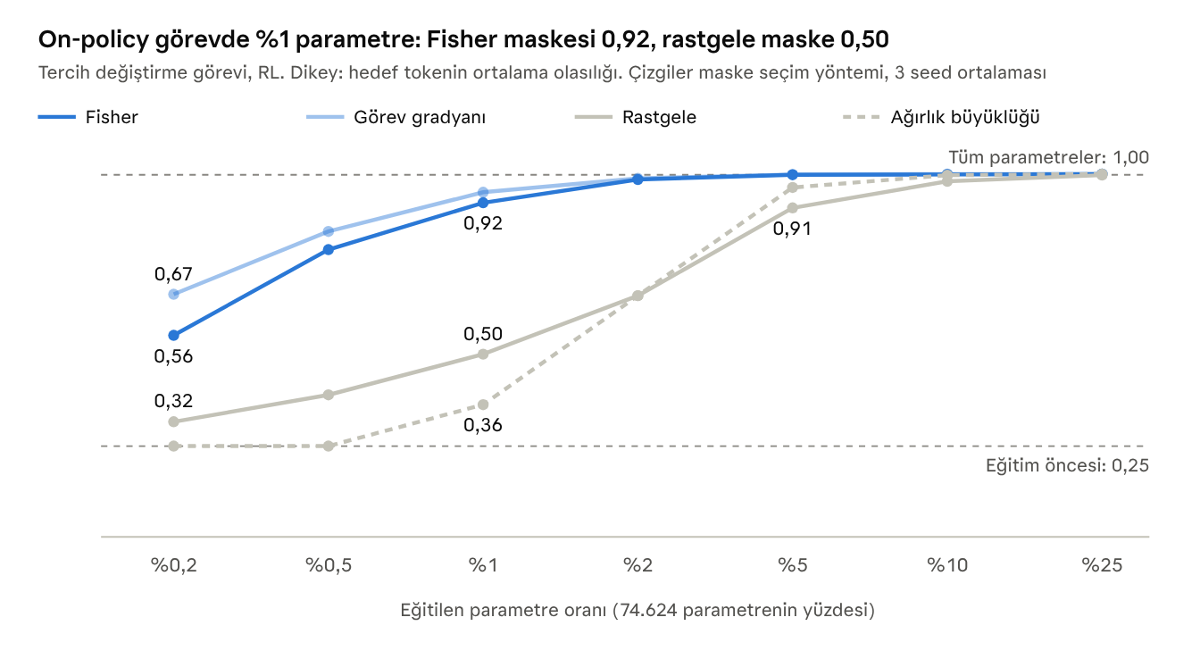
Paper A’s second claim holds too: at a 1% parameter budget, the Fisher mask recovers 90% of full-training improvement (0.92 versus full training’s 1.00, starting at 0.25), while random masking recovers 34%. The paper’s real-model figures are 96% and 25%.
Two results are absent from the paper.
Task-gradient scoring beats Fisher at every budget. The gap is clearest at the smallest budget (0.67 versus 0.56) and closes with larger budgets. This makes Section 4.4’s criticism concrete: Fisher is not special; a task-aware score is at least as good. Fisher’s only advantage is requiring no task data.
Weight magnitude is worse than random. At a 0.5% budget, magnitude masking learns nothing (0.25), while random reaches 0.39. Large weights matter to the model’s current behavior, not necessarily to the change needed. This agrees with Paper C’s finding that RL avoids principal weights.
One difference from real models: random masks improve smoothly with budget here instead of remaining flat at the base level as in Paper B. Section 9.3 discusses this.
8.4 Test 3: Fisher masks when teaching something new
We test the same four masks on teaching a token the model has never produced.
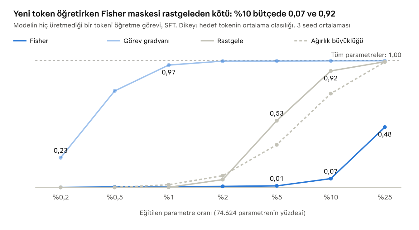
This is the section’s clearest result. Even training 10% of parameters, Fisher masking stays at 0.07; random masking reaches 0.92 at the same budget. Task-gradient masking reaches 0.97 with just 1%. Fisher does more than fail: it systematically looks in the wrong place. The necessary weights are precisely those it calls “unimportant.”
This result appears in none of the three papers but connects all of them.
Paper A’s loose off-policy bound can, in practice, mean Fisher selection reverses its usefulness. The authors’ caution against proposing it as a general method is justified and important.
Paper B’s unexplained GPQA anomaly—Fisher scoring at base level while gradient scoring and random selection improve—may be a real-model trace of this. That SFT experiment used data far from the model’s distribution. This is a hypothesis: since its score uses task loss, the mechanism may not be identical.
This is the masking counterpart to the blog’s statement that editing removes barriers rather than adds capabilities: weights selected using the model’s own sensitivities can reweight existing behaviors rather than construct new ones.
Practical implication: for sparse post-training mask selection, task-gradient scoring such as Paper B’s Ŝ is the only option working in both cases here. Fisher is safe only when the task is known to be on-policy.
8.5 Test 4: the SFT/RL difference
To test Paper B’s main claim, we train the same preference-shifting task with both RL and SFT. The claim does not hold: mask rankings and gaps are almost identical across regimes.
| 1% budget | Fisher | Task gradient | Random |
|---|---|---|---|
| RL | 0.92 | 0.95 | 0.50 |
| SFT | 0.91 | 0.94 | 0.48 |
Gradient structure explains why. We compute Paper B’s three metrics over 64 minibatch gradients:
| Metric | SFT | RL | Paper B (Qwen2.5-1.5B, SFT / GRPO) |
|---|---|---|---|
| Cross-step cosine | 0.11 | 0.08 | 0.76 / 0.04 |
| Effective rank | 30 | 35 | 2.6 / 21.8 |
| Accumulation efficiency | 0.35 | 0.31 | 0.90 / 0.28 |
The toy model’s RL values resemble the real model’s. SFT differs: real-model SFT gradients point similarly across steps (0.76), ours do not (0.11). The reason is clear: each context in our model has its own embedding row, so different minibatches touch different parameters. In a real language model all SFT examples pass through shared weights and jointly push a common direction, such as an answer format.
This negative result is informative. Paper B’s SFT/RL contrast is not an intrinsic mathematical property of the regimes; it depends on shared structure across SFT examples. If data is heterogeneous and each example teaches something different, SFT can behave like RL and placement can matter there too. The paper’s instruct-model exception and sparse-B deficit on difficult SFT (GPQA) are consistent with this reading.
One measure does agree with the paper. Across all coordinates, mean absolute gradient-sign consistency over 64 minibatches is 0.36 for SFT and 0.04 for RL. SFT applies a small, consistent push per parameter; RL gives most parameters random-sign noise. Among the top 1% by gradient, however, the regimes are similar (0.18 and 0.19).
8.6 Test 5: collateral damage
KL drift on contexts never used for training, in the preference-shifting task:
| Method | RL success | RL damage | SFT success | SFT damage |
|---|---|---|---|---|
| All parameters | 1.00 | 0.41 | 1.00 | 2.19 |
| Fisher mask, 5% | 1.00 | 0.04 | 1.00 | 0.03 |
| Task-gradient mask, 5% | 1.00 | 0.09 | 1.00 | 0.07 |
| Random mask, 5% | 0.91 | 0.25 | 0.90 | 0.58 |
| Weight-magnitude mask, 5% | 0.96 | 0.41 | 0.96 | 1.01 |
Three observations follow.
A well-selected sparse mask causes ten times less damage at equal success. A 5% Fisher mask matches full training while reducing drift from 0.41 to 0.04. This agrees with Paper C’s forgetting result and adds something it did not establish: deletion itself may not be what reduces forgetting; a small, well-targeted set of modified weights may suffice. Paper C lacked the ablation to distinguish them.
Sparsity alone is insufficient. Random and magnitude masks cause six to ten times more damage at equal budgets. As with Paper C’s rank-1 LoRA forgetting more than FFT, the lesson is to choose the right parameters rather than merely fewer parameters.
SFT produces five times the drift of RL at equal success (2.19 versus 0.41). This follows directly from Paper A’s signal-scale factor. RL’s signal is reward variance, naturally approaching zero as the model succeeds; RL is self-limiting. SFT keeps pushing for the remaining 1% even when the target already has 99% probability. This comparison is not entirely fair—early stopping SFT would narrow the gap—but the mechanism is real.
8.7 Test 6: learning through deletion alone
We test Paper C’s idea in its simplest form: frozen weights, one logit per weight, a hard forward-pass mask, and straight-through gradients. This is not the paper’s parameterization, which uses soft masks and Wanda initialization, so the result should be read as a lower-bound demonstration.
| Setting | Weights deleted | Success (initially 0.25) | Collateral damage |
|---|---|---|---|
| Sparsity penalty, embedding excluded | 0.2–0.5% | 0.43–0.44 | 0.07–0.19 |
| Sparsity penalty, embedding included | 0.3–0.6% | 0.57–0.61 | 0.04–0.11 |
| No sparsity penalty, embedding included | 31% | 1.00 | 2.20 |
Deletion alone can solve the task, but requires removing a third of weights and causes more damage than FFT. Deleting a few tenths of a percent recovers between a quarter and half the gain. At this scale, the “0.05% suffices” result does not emerge.
This fits Paper C’s small-model deficit and Section 6.6’s redundancy hypothesis: a 75,000-parameter model has almost no spare capacity to delete. But our setup is crude and covers one architecture; the result is better described as not contradicting the hypothesis than supporting it.
8.8 A mechanism that did not hold: token sensitivities
Paper A explains small Fisher through likely tokens responding similarly to a parameter, reporting an actual/uniform variance ratio of 0.16. Computing the same ratio for our hidden-layer neurons gives 1.26, above one: likely tokens respond more differently than random tokens.
This is informative too. The token-level mechanism comes from real language structure rather than softmax mathematics. Plausible continuations in real language are semantically related—tea, coffee, water—and have similar output vectors. In our artificial language, the five plausible tokens were selected randomly and share no similarity. This part of sparsity is an empirical property of language models.
8.9 Balance sheet
| Claim | Source | Toy-model result | Interpretation |
|---|---|---|---|
| Fisher bounds expected gradients | A | Holds, zero violations; very loose bound | Mathematical necessity |
| Fisher locates gradients on-policy, not off-policy | A | Holds: hit rate falls from 58% to 14% | Appears architecture-independent |
| Fisher masks outperform random masks on-policy | A | Holds: 0.92 versus 0.50 at 1% | Appears architecture-independent |
| Placement matters in RL but not SFT | B | Does not hold: matters in both | Depends on shared SFT-data structure |
| Random placement never learns in RL | B | Does not hold: learns slowly | Depends on scale and noise |
| Very little deletion matches full training | C | Does not hold: partial gain | Requires redundancy; scale-dependent |
| Sparse, well-targeted updates forget less | C | Holds: tenfold lower collateral damage | May not be specific to deletion |
| Likely tokens have similar sensitivities | A | Does not hold: ratio 1.26 | A property of real language |
| Fisher masks fail when teaching new behavior | New | Worse than random | Should be tested in a real model |
9. Synthesis: what the three papers say together
The papers agree on four points and diverge on three. One disagreement—whether random sparse selection works—is discussed by none of them and emerges only when they are read side by side.
9.1 Side by side
| A: Fisher perspective | B: LoRA placement | C: Deletion Tuning | Blog: WSP | |
|---|---|---|---|---|
| Question | Why sparse? | Which parameters? | How few suffice? | Are gradients necessary? |
| Selection | Before training; Fisher from the model’s own samples | Before training; task gradients from 50 passes | Learned during training; Wanda initialization | Model reasoning and a few forward passes |
| Operation | Freely train selected weights | Train selected LoRA-B entries | Delete gate weights | Subtract a direction or write weights directly |
| Fraction affected | 0.05–5% of all weights | 1,000–100,000 entries | Less than 0.05% of all weights | 0.016% in the Qwen case |
| Models | Qwen3-1.7B base | Qwen2.5 1.5B–7B base; Llama 3B–8B instruct | Llama 1B–8B instruct; Qwen2.5 0.5B–14B base; Qwen3 30B MoE | Qwen3.5-0.8B and small networks |
| Regimes | RL, OPD | SFT, GRPO | GRPO, SFT, OPD | No training |
| Forgetting measured? | No | No | Yes, after one task | No |
| Compute savings | Not demonstrated | Not demonstrated | Storage savings, not training savings | Not applicable |
| Weakest point | One model; random-only baseline | Contrast specific to base models | Missing ablations; trails below 7B | Case-level evidence |
9.2 Four points of agreement
On-policy signal falls on few coordinates. A establishes this theoretically; B measures it (0.05% of entries carry 8–15% of gradient energy); C exploits it. Three independent teams, three methods, one phenomenon.
These coordinates can be found cheaply before training. A needs 800 questions with one model answer each; B needs 50 forward-backward passes and under 10 seconds. The scores belong to the same family: B’s F̂ is a Fisher estimate, and A’s bound limits B’s Ŝ.
The change adjusts use of existing capabilities rather than adding them. C’s pass@k table—the base solves 95% of questions in 128 attempts—the blog’s negative result with a non-looping model, and our Test 3, in which Fisher masking cannot teach a new token, express the same point in three ways.
The affected weights are not the largest or most central. C’s RL updates have below-random principal-weight overlap. Our magnitude-selected masks are worse than random. Post-training touches secondary connections rather than the model’s backbone.
9.3 Three disagreements
Disagreement 1: does random sparse selection work?
| Paper | Setup | Random selection | Full training | Initial |
|---|---|---|---|---|
| A | Qwen3-1.7B base, random 0.05%, MATH-500 | 23.21 | 56.41 | 22.65 |
| B | Qwen2.5-1.5B base, 10,000 random LoRA-B entries, GSM8K | 9.8 | 62.8 | 9.5 |
| C | Qwen2.5-7B base, random 0.05% (MTH), six benchmarks | 51.24 | 51.89 | Not recorded in this reading |
| C | Qwen2.5-0.5B base, random 0.05% (MTH) | 20.16 | 19.01 | Not recorded in this reading |
In A and B, random selection learns nothing. In C, with the same fraction, model family, and base-model setting, it matches FFT and exceeds it at 0.5B. None discusses this gap because each considers only its own random baseline.
Three possible explanations follow, all our interpretations.
Learning rate. A uses the same learning rate for masked training and FFT (5e-7); B uses 1e-6. Under Adam, a parameter’s step depends on learning rate rather than gradient magnitude; in 1,000 steps a parameter can move only on the order of a thousandth. Such movement affects output only in a sensitive, high-Fisher parameter. A random subset moves at this learning rate without leaving a trace. A separately tuned sparse baseline could compensate with a higher rate. We do not know C’s MTH learning rate.
Budget. B uses at most 50,000 entries. In C, 0.05% of a 7B model is about 3.8 million weights, over a hundred times more. Our random masks also improve smoothly with budget, from 0.32 to 0.91, without a sharp failure.
Scale. C’s random baseline works in a large model; redundancy increases the chance that a random subset contains useful weights. But the 0.5B result weakens this explanation.
We consider the first strongest. If correct, A and B’s claim should become “informed selection is much more efficient at the same learning rate and budget,” rather than “random selection does not learn.” This is weaker but more defensible. Section 11’s first experiment tests it.
Disagreement 2: should gate be the target?
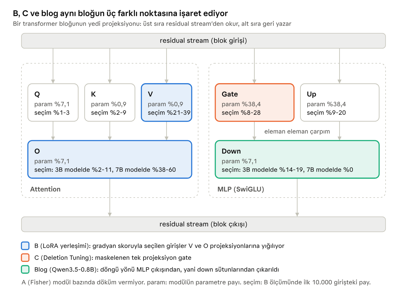
B finds that gradient-based selection underrepresents gate relative to its parameter share, explaining that gate does not write directly to the residual stream. C targets only gate and matches FFT. Both can be true because they measure different things.
The operations differ. In B, a gate entry is an additive correction in a subspace defined by frozen random A. In C, it deletes one actual weight. “LoRA-B gate entries receive little gradient” is not equivalent to “deleting individual gate weights does not work.”
The score is scale-sensitive. B globally selects across modules using raw gradient magnitude. Gate gradients pass through an activation derivative and multiplication by up, potentially reducing magnitude. B’s appendix says gate’s sign consistency matches V and O. Gate may be underselected because its gradients are small, not because it is unimportant. C’s optimizer takes a scale-independent step per logit.
C never tested the alternative. Deleting V or O weights might outperform gate. B suggests the experiment is worth running.
Disagreement 3: what happens in SFT?
B says placement is unimportant in SFT. A says SFT is sparse only when its data is close to the model. C’s OPD requires four to seven times as much deletion as RL. Our experiment finds no SFT/RL difference. These observations cannot be reconciled along an “SFT versus RL” axis; that is not the right axis.
Our proposed reading is that two properties, rather than the regime’s name, are decisive.
| Signal consistent across examples | Signal noisy or heterogeneous across examples | |
|---|---|---|
| Signal close to the model’s distribution | Sparse update; placement matters less. Example: near-policy SFT | Sparse update; placement is decisive. Example: RL, B’s base-model results |
| Signal far from the model’s distribution | Dense update; any subset accumulates, but capacity is needed. Example: B’s Alpaca and GPQA results | Hardest case; Fisher misleads and task gradients are needed. Example: our new-token task |
The first axis is A’s chi-squared term; the second is B’s cross-step cosine. RL always occupies the upper-right cell; SFT can occupy any cell depending on its data. B’s “unimportant in SFT” result belongs to the left column, while our “important in SFT too” result belongs to the right.
9.4 A short derivation connecting A and B
A considers expected gradient magnitude; B considers sign consistency. Writing down Adam’s operation shows how they connect. This heuristic derivation is ours.
Adam divides each coordinate’s mean gradient by its root second moment. Over T steps, total displacement is approximately learning rate times step count times signal-to-noise ratio:
The resulting effect on the output distribution depends on sensitivity, the square root of Fisher. For a bounded signal such as binary reward, the gradient’s second moment is roughly proportional to Fisher, so the square roots cancel:
Thus, under Adam a coordinate’s contribution to model behavior is proportional to its absolute expected gradient—exactly B’s Ŝ score. A’s inequality bounds that quantity through Fisher.
This explains three observations. First, why Ŝ and F̂ perform similarly, but Ŝ is more reliable at small budgets and on the difficult task: F̂ measures a bound, Ŝ the quantity itself. Second, why our task-gradient mask beats Fisher at every budget. Third, why Fisher collapses off-policy: an unbounded signal breaks the proportionality between second moment and Fisher, making the bound uninformative.
Practically, if one score must be chosen for sparse post-training, it is the absolute initial mean task gradient. Fisher is a proxy when task data is unavailable and is reliable only for on-policy tasks.
10. Open questions
The papers and Section 8’s experiment leave six questions unanswered. For each we state what the evidence predicts and what result would falsify it. All predictions are ours.
10.1 What if the same weights must be preserved and changed?
This is the tension from Section 2.5. Elastic Weight Consolidation protects high-Fisher weights as important to old tasks. Paper A shows on-policy updates falling precisely on those weights. Mukherjee and colleagues also found RL subnetworks overlapping across datasets and algorithms far more than chance.
Together these suggest an uncomfortable prediction: sequential RL tasks will demand many of the same coordinates. C’s low forgetting was measured on previous tasks quite different from its RL task—general knowledge, code, instruction following. With two similar RL tasks in sequence, the second mask may need weights the first deleted.
Prediction: masks for two RL tasks overlap far above chance, and their union performs worse on both tasks than each separate mask.
Falsifying result: masks are disjoint and their union preserves both tasks. Mask algebra—union, intersection, subtraction—would then be a megabyte-scale counterpart of task-vector arithmetic. C lists combining masks by union as untested future work.
10.2 Where is the lower limit of redundancy?
C falls behind below 7B. Our 75,000-parameter model needs one-third of its weights deleted to solve the task through deletion alone. Somewhere lies a transition from “deletion suffices” to “deletion does not suffice,” determining usefulness for small-language-model practitioners.
Two things remain unknown. First, whether the deficit reflects model size or a narrow target: C masks only gate, whereas B locates concentrated signal in V and O. Second, base versus instruct: C’s small Llama models are instruct, and B shows instruction tuning changes gradient structure.
Prediction: expanding deletion candidates to V and O substantially narrows the 1B–3B deficit.
Falsifying result: the deficit persists regardless of target. The limit would then genuinely concern capacity, and deletion could not replace unrestricted training in small models.
10.3 Can selection and deletion be combined?
C’s training cost comes from maintaining one logit per gate weight—about 1.9 billion in an 8B model. B finds candidate weights in 10 seconds. They naturally complement each other: first select 100,000–1 million candidates by task gradient, then train only their logits. C’s authors mention candidate restriction but do not specify a score.
Prediction: equal accuracy with a thousand times fewer trainable logits. If Section 6.7’s saturated-sigmoid reading is correct, this already happens implicitly, with Wanda and noise determining candidates.
Falsifying result: accuracy drops when candidates are restricted. Weights needing deletion would then emerge during training rather than being predictable from initial gradients.
10.4 How much sparsity comes from the optimizer?
A bounds expected gradients, but the observed phenomenon—most weights never changing—passes through the optimizer, learning rate, and numerical precision. Since Adam normalizes gradient magnitude, a small gradient alone does not imply a small step. Section 9.3’s random-baseline contradiction points to the same issue.
Section 9.4 suggests a distinction: functionally important coordinates may be optimizer-independent, while the count changing measurably depends on learning rate and threshold.
Prediction: with SGD or a tenfold learning rate, the unchanged-weight fraction drops substantially, while the top 1% of changed coordinates stays largely the same.
Falsifying result: the top-changed set varies by optimizer. “RL trains this subnetwork” would then mean “RL with Adam trains this subnetwork.”
10.5 Can the changes be read?
The blog attempts to read entire networks and reaches a limit around 7 million parameters. Yet these three papers show the post-training change is a small object: 10,000 entries in B, a mask of a few megabytes in C. Reading only the difference may be a more realistic application. “What did RL change in this model?” becomes a table of ten thousand rows.
C’s stable rank of 66–93 says the difference is neither one direction nor unstructured scatter; B’s ablation says selected entries are causal. The remaining question is whether they cluster into meaningful units such as particular neurons or heads.
Prediction: deleted or selected weights concentrate in a small set of neurons and heads, some with nameable functions.
Falsifying result: weights are spread across units, none independently meaningful. Sparsity would then not confer interpretability.
10.6 What does a new capability require?
Nearly all the evidence concerns reweighting existing capabilities. Three clues address genuinely new learning. Our task-gradient mask teaches a new token at 1%, whereas Fisher does not. B’s sparse B trails full LoRA by seven points on difficult SFT. C’s distillation needs four to seven times more deletion than RL.
Prediction: off-policy learning can use sparse updates but needs at least ten times the on-policy budget, selected using task gradients.
Falsifying result: real-model off-policy learning matches full training below a 0.1% budget. Sparsity would then not be specific to on-policy learning, and A’s framework would be too narrow.
11. Six experiments to test these questions
For each disagreement and question in Sections 9 and 10, we define the smallest experiment capable of answering it. All share a base setup so results can be compared.
Shared setup. Qwen2.5-1.5B base, GRPO on MATH, evaluated on GSM8K and MATH-500. This is B’s sharpest setting: base 9.5%, full LoRA 62.8%, a gap large enough to expose methodological differences. The model fits on one 16 GB GPU.
| No. | Question tested | Arms | Decision criterion |
|---|---|---|---|
| D1 | Does random sparse selection fail, or is the learning rate insufficient? (9.3, disagreement 1) | Random 0.05% of all weights versus task-gradient-selected 0.05%, each at four learning rates: 1e-6, 1e-5, 1e-4, 1e-3 | If any random-mask learning rate recovers over half the full-training improvement, A and B’s claim depends on learning rate |
| D2 | Gate or V/O; deletion or training? (9.3, disagreement 2) | Equal counts of actual weights in four arms: train gate, train V/O, delete gate, delete V/O | A 2×2 table separates operation effects (rows) from target effects (columns) |
| D3 | Is early-layer concentration functional or a scale artifact? (5.6) | B’s global selection versus selection normalized by each matrix’s gradient norm, equal budgets | If normalization spreads the budget across layers without losing accuracy, concentration is an artifact |
| D4 | Does Fisher masking collapse off-policy in a real model? (8.4) | SFT on an unfamiliar format or knowledge; Fisher, task-gradient, and random masks at 0.1% | Fisher below random would validate Section 8.4 at real-model scale |
| D5 | Do sequential-task masks overlap? (10.1) | Two sequential RL tasks; separate masks, overlap, union, and sequential training | If overlap exceeds ten times chance and union harms both tasks, low forgetting does not transfer to similar tasks |
| D6 | How many logits actually train in Deletion Tuning? (6.7, 10.3) | Reimplement on 0.5B; logit histograms and stepwise mask turnover; another arm restricts logits to task-gradient candidates | If all sign-changing logits start near threshold, noise determines the candidate set |
Priority: D1, D4, D2. D1 is cheapest and determines the scope of two papers’ main claim. D4 tests this article’s finding at real scale. D2 is most informative but needs four arms.
An implementation note for D2: B measures LoRA-B entries; C measures actual weights. To compare the four arms, all must operate on actual weights, with selection performed separately within each module. Otherwise Section 9.3’s scale issue enters the experiment.
12. Limitations of this article
Reading method. All three papers were read in full through text extraction. Values inside figures—A’s Figure 3 and C’s Figures 2 and 3—were used only where repeated in the text. B’s internal inconsistencies were not visually checked in the original PDF.
Unknowns. C’s MTH learning rate and covered modules are unknown; Section 9.3’s first explanation depends on them. Without mask-initialization details from C’s Equation 8, the saturated-sigmoid interpretation remains qualitative.
Our experiment’s scale. Section 8’s model has 75,000 parameters, no attention, and an artificial language. Results illuminate mechanisms without establishing conclusions about real models. There are three seeds and no confidence intervals.
Interpretations. Anything marked “our reading,” “hypothesis,” or “prediction” is an untested inference. Section 9.4’s heuristic derivation ignores Adam’s momentum and epsilon terms and correlations between gradients.
Background sources. Classic studies in Sections 2 and 3 were discussed from general knowledge rather than reread for this article. Their arXiv links and titles were checked before publication.
The blog post. It is not peer-reviewed; we know no more about its Astra model than the post provides.
Glossary
| Term | In one sentence | First appearance |
|---|---|---|
| Post-training | Any training after pretraining: SFT, RL, distillation | 2.2 |
| On-policy, off-policy | On-policy data comes from the model’s own answers; off-policy data comes from outside | 2.2 |
| GRPO | An RL algorithm rewarding answers to one question relative to other answers in their group | 2.2 |
| Residual stream | The shared vector flowing through the model that each layer reads and writes | 2.3 |
| Projection | A block’s linear layers: Q, K, V, O, gate, up, down | 2.3 |
| LoRA | A trainable low-rank correction added alongside frozen weights | 2.4 |
| Fisher | A measure of how much perturbing a parameter changes the output distribution | 2.5 |
| Score | The derivative of a sampled answer’s log-probability with respect to a parameter | 2.5 |
| Mask | A binary table specifying which weights to train or delete | 3.2 |
| Baseline | A reference method for comparison; in RL, also the mean subtracted from rewards | 4.3 |
| Circuit | In B, score-selected entries; more generally, a weight subset implementing a task | 5.2 |
| Base, instruct | A model with pretraining only; one additionally trained to follow instructions | 5.3 |
| pass@k | The fraction of problems with at least one correct answer in k attempts | 6.3 |
| Stable rank | A noise-robust rank measure indicating how many directions carry matrix energy | 6.5 |
References
Primary sources
Zhang, Mukherjee, Peng. Understanding LLM Parameter Update Sparsity through the Lens of Fisher. arXiv:2609.36262, 2026.
Sehanobish, Lovering. Not How Many, But Which: Parameter Placement in Low-Rank Adaptation. arXiv:2605.12207, 2026.
Lu, Yang, Lasby, Pote, Ioannou, Ren. The Surprising Effectiveness of Deleting Weights in LLM Post-Training. NeurIPS 2026, arXiv:2611.10866.
Takehi, Teoh, Zhang, Khattab. Sparks of Weight-Space Programming. MIT CSAIL blog, 2 November 2026.
Direct predecessors
Mukherjee, Yuan, Hakkani-Tür, Peng. Reinforcement Learning Finetunes Small Subnetworks in Large Language Models. NeurIPS 2025.
Zhu and colleagues. The Path Not Taken: RLVR Learns Off the Principals. NeurIPS 2026. (Cited by Paper C.)
Adewuyi and colleagues. Multiple Ticket Hypothesis. 2026. (Cited by Paper C.)
Pruning and mask learning
LeCun, Denker, Solla. Optimal Brain Damage. NIPS 1989.
Hassibi, Stork. Second Order Derivatives for Network Pruning: Optimal Brain Surgeon. NIPS 1993.
Han and colleagues. Learning both Weights and Connections for Efficient Neural Networks. 2015.
Lee, Ajanthan, Torr. SNIP: Single-shot Network Pruning based on Connection Sensitivity. 2018.
Frankle, Carbin. The Lottery Ticket Hypothesis. 2018.
Mallya, Davis, Lazebnik. Piggyback: Adapting a Single Network to Multiple Tasks by Learning to Mask Weights. 2018.
Zhou, Lan, Liu, Yosinski. Deconstructing Lottery Tickets: Zeros, Signs, and the Supermask. 2019.
Ramanujan and colleagues. What's Hidden in a Randomly Weighted Neural Network?. 2019.
Malach and colleagues. Proving the Lottery Ticket Hypothesis: Pruning is All You Need. 2020.
Zhao and colleagues. Masking as an Efficient Alternative to Finetuning for Pretrained Language Models. 2020.
Sanh, Wolf, Rush. Movement Pruning: Adaptive Sparsity by Fine-Tuning. 2020.
Guo, Rush, Kim. Parameter-Efficient Transfer Learning with Diff Pruning. 2020.
Sung, Nair, Raffel. Training Neural Networks with Fixed Sparse Masks. 2021.
Sun, Liu, Bair, Kolter. A Simple and Effective Pruning Approach for Large Language Models. 2023.
Weight space and model editing
Kirkpatrick and colleagues. Overcoming Catastrophic Forgetting in Neural Networks. 2017.
Li and colleagues. Measuring the Intrinsic Dimension of Objective Landscapes. 2018.
Aghajanyan, Zettlemoyer, Gupta. Intrinsic Dimensionality Explains the Effectiveness of Language Model Fine-Tuning. 2020.
Meng and colleagues. Locating and Editing Factual Associations in GPT. 2022.
Ilharco and colleagues. Editing Models with Task Arithmetic. 2022.
Lindner and colleagues. Tracr: Compiled Transformers as a Laboratory for Interpretability. 2023.
Arditi and colleagues. Refusal in Language Models Is Mediated by a Single Direction. 2024.